In ZellW/LearnPlotting:

knitr::opts_chunk$set(echo = TRUE)

I will show you how to use text data to build word clouds in R. I saved all the AWE Basecamp discussions to a Word file. I then save the Word file as text.

We will require three packages for this: tm, SnowballC, and wordcloud.

First, let’s load the required libraries and read in the data.

library(tm)
library(SnowballC)
library(wordcloud)

jeopQ <- read.csv("../data/Words/BasecampArchive.txt", stringsAsFactors = FALSE)

Now, we will perform a series of operations on the text data to simplify it. First, we need to create a corpus.

jeopCorpus <- Corpus(VectorSource(jeopQ))

Next, we will convert the corpus to a plain text document.

jeopCorpus <- tm_map(jeopCorpus, PlainTextDocument)

Then, we will remove all punctuation and stopwords. Stopwords are commonly used words in the English language such as I, me, my, etc. You can see the full list of stopwords using stopwords('english'). I also selectively removed the and this.

jeopCorpus <- tm_map(jeopCorpus, removePunctuation)
jeopCorpus <- tm_map(jeopCorpus, removeWords, c('october', 'can', 'will', 'post', 'just', 'the', 'this', '2015', stopwords('english')))

Next, we will perform stemming. This means that all the words are converted to their stem (Ex: learning -> learn, walked -> walk, etc.). This will ensure that different forms of the word are converted to the same form and plotted only once in the wordcloud.

jeopCorpus <- tm_map(jeopCorpus, stemDocument)

Now, we will plot the wordcloud.

wordcloud(jeopCorpus, max.words = 100, random.order = FALSE, colors = brewer.pal(5,"Greens"))

There are a few ways to customize it.

scale: This is used to indicate the range of sizes of the words.
max.words and min.freq: These parameters are used to limit the number of words plotted. max.words will plot the specified number of words and discard least frequent terms, whereas, min.freq will discard all terms whose frequency is below the specified value.
random.order: By setting this to FALSE, we make it so that the words with the highest frequency are plotted first. If we don’t set this, it will plot the words in a random order, and the highest frequency words may not necessarily appear in the center.
rot.per: This value determines the fraction of words that are plotted vertically.
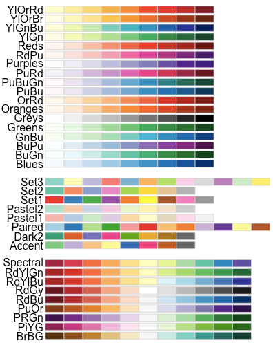
colors: The default value is black. If you want to use different colors based on frequency, you can specify a vector of colors, or use one of the pre-defined color palettes. You can find a list here.

There is an even easier way! See here.

The following packages are required for the rquery.wordcloud() function:

tm for text mining
SnowballC for text stemming
wordcloud for generating word cloud images
RCurl and XML packages to download and parse web pages
RColorBrewer for color palettes

If needed, install these packages, before using the function rquery.wordcloud, as follows:

install.packages(c("tm", "SnowballC", "wordcloud", "RColorBrewer", "RCurl", "XML")

library(tm)
library(SnowballC)
library(wordcloud)
library(RCurl)
library(XML)

source('http://www.sthda.com/upload/rquery_wordcloud.r')

The format of rquery.wordcloud() function is shown below :

rquery.wordcloud(x, type=c("text", "url", "file"), 
        lang="english", excludeWords = NULL, 
        textStemming = FALSE,  colorPalette="Dark2",
        max.words=200)

Let's run it:

#Let's create a list of excluded words
badWords <- c("also", "see", "may", "using", "make", "can", "will", "want", "know", "posted", "really", "october")
res<-rquery.wordcloud("../data/Words/BasecampArchive.txt", type ="file", lang = "english", min.freq = 5, max.words = 100,
                      excludeWords = badWords)

Here are the parameters:

x: character string (plain text, web URL, txt file path)
type: specify whether x is a plain text, a web page URL or a .txt file path
lang: the language of the text. This is important to be specified in order to remove the common stopwords (like ‘the’, ‘we’, ‘is’, ‘are’) from the text before further analysis. Supported languages are danish, dutch, english, finnish, french, german, hungarian, italian, norwegian, portuguese, russian, spanish and swedish.
excludeWords: a vector containing your own stopwords to be eliminated from the text. e.g : c(“word1”, “word2”)
textStemming: reduces words to their root form. Default value is FALSE. A stemming process reduces the words “moving” and “movement” to the root word, “move”.
colorPalette: Possible values are : ◦a name of color palette taken from RColorBrewer package (e.g.: colorPalette = “Dark2”)
- color name (e.g. : colorPalette = “red”) +a color code (e.g. : colorPalette = “#FF1245”)
min.freq: words with frequency below min.freq will not be plotted
max.words: maximum number of words to be plotted. least frequent terms dropped

Note rquery.wordcloud() function returns a list, containing two objects: tdm: term-document matrix which can be explored as illustrated in the next sections. freqTable: Frequency table of words

Change the arguments max.words and min.freq to plot more words:

max.words: maximum number of words to be plotted.
min.freq: words with frequency below min.freq will not be plotted

res<-rquery.wordcloud("../data/Words/BasecampArchive.txt", type ="file", lang = "english", min.freq = 3,  max.words = 200,
                      excludeWords = badWords)

Change the color of the word cloud

The color of the word cloud can be changed using the argument colorPalette.

Allowed values for colorPalete:

a color name (e.g.: colorPalette = “blue”)
a color code (e.g.: colorPalette = “#FF1425”)
a name of a color palette taken from RColorBrewer package (e.g.: colorPalette = “Dark2”)

# Reds color palette
res <- rquery.wordcloud("../data/Words/BasecampArchive.txt", type ="file", lang = "english",
                      colorPalette = "Reds", excludeWords = badWords)

# RdBu color palette
res<-rquery.wordcloud("../data/Words/BasecampArchive.txt", type ="file", lang = "english",
                      colorPalette = "RdBu", excludeWords = badWords)

# use unique color
res<-rquery.wordcloud("../data/Words/BasecampArchive.txt", type ="file", lang = "english",
                      colorPalette = "black", excludeWords = badWords)

Operations on the result of rquery.wordcloud() function

As mentioned above, the result of rquery.wordcloud() is a list containing two objects:

tdm : term-document matrix
freqTable : frequency table

tdm <- res$tdm
freqTable <- res$freqTable

Frequency table of words

The frequency of the first top words can be displayed and plotted as follows:

# Show the top10 words and their frequency
head(freqTable, 10)

# Bar plot of the frequency for the top10
barplot(freqTable[1:10,]$freq, las = 2, names.arg = freqTable[1:10,]$word,
        col ="lightblue", main ="Most frequent words", ylab = "Word frequencies")

Operations on term-document matrix

You can explore the frequent terms and their associations. In the following example, we want to identify words that occur at least four times:

findFreqTerms(tdm, lowfreq = 20)

You could also analyze the correlation (or association) between frequent terms. The R code below identifies which words are associated with “campaign”:

findAssocs(tdm, terms = "campaign", corlimit = 0.3)

Create a word cloud of a web page

In this section we’ll make a tag cloud of the following web page :

http://www.sthda.com/english/wiki/create-and-format-powerpoint-documents-from-r-software

url = "http://www.sthda.com/english/wiki/create-and-format-powerpoint-documents-from-r-software"
rquery.wordcloud(x=url, type="url")

< The above word cloud shows that “powerpoint”, “doc”, “slide”, “reporters” are among the most important words on the analyzed web page. This confirms the fact that the article is about creating PowerPoint document using ReporteRs package in R

R code of rquery.wordcloud function

#++++++++++++++++++++++++++++++++++
# rquery.wordcloud() : Word cloud generator
# - http://www.sthda.com
#+++++++++++++++++++++++++++++++++++
# x : character string (plain text, web url, txt file path)
# type : specify whether x is a plain text, a web page url or a file path
# lang : the language of the text
# excludeWords : a vector of words to exclude from the text
# textStemming : reduces words to their root form
# colorPalette : the name of color palette taken from RColorBrewer package, 
  # or a color name, or a color code
# min.freq : words with frequency below min.freq will not be plotted
# max.words : Maximum number of words to be plotted. least frequent terms dropped

# value returned by the function : a list(tdm, freqTable)
rquery.wordcloud <- function(x, type=c("text", "url", "file"), 
                          lang="english", excludeWords=NULL, 
                          textStemming=FALSE,  colorPalette="Dark2",
                          min.freq=3, max.words=200)
{ 
  library("tm")
  library("SnowballC")
  library("wordcloud")
  library("RColorBrewer") 

  if(type[1]=="file") text <- readLines(x)
  else if(type[1]=="url") text <- html_to_text(x)
  else if(type[1]=="text") text <- x

  # Load the text as a corpus
  docs <- Corpus(VectorSource(text))
  # Convert the text to lower case
  docs <- tm_map(docs, content_transformer(tolower))
  # Remove numbers
  docs <- tm_map(docs, removeNumbers)
  # Remove stopwords for the language 
  docs <- tm_map(docs, removeWords, stopwords(lang))
  # Remove punctuations
  docs <- tm_map(docs, removePunctuation)
  # Eliminate extra white spaces
  docs <- tm_map(docs, stripWhitespace)
  # Remove your own stopwords
  if(!is.null(excludeWords)) 
    docs <- tm_map(docs, removeWords, excludeWords) 
  # Text stemming
  if(textStemming) docs <- tm_map(docs, stemDocument)
  # Create term-document matrix
  tdm <- TermDocumentMatrix(docs)
  m <- as.matrix(tdm)
  v <- sort(rowSums(m),decreasing=TRUE)
  d <- data.frame(word = names(v),freq=v)
  # check the color palette name 
  if(!colorPalette %in% rownames(brewer.pal.info)) colors = colorPalette
  else colors = brewer.pal(8, colorPalette) 
  # Plot the word cloud
  set.seed(1234)
  wordcloud(d$word,d$freq, min.freq=min.freq, max.words=max.words,
            random.order=FALSE, rot.per=0.35, 
            use.r.layout=FALSE, colors=colors)

  invisible(list(tdm=tdm, freqTable = d))
}

#++++++++++++++++++++++
# Helper function
#++++++++++++++++++++++
# Download and parse webpage
html_to_text<-function(url){
  library(RCurl)
  library(XML)
  # download html
  html.doc <- getURL(url)  
  #convert to plain text
  doc = htmlParse(html.doc, asText=TRUE)
 # "//text()" returns all text outside of HTML tags.
 # We also don’t want text such as style and script codes
  text <- xpathSApply(doc, "//text()[not(ancestor::script)][not(ancestor::style)][not(ancestor::noscript)][not(ancestor::form)]", xmlValue)
  # Format text vector into one character string
  return(paste(text, collapse = " "))
}